Survival Curves for Financial Planning

Stanislav Traykov

2026-01-08

Setup

library(fundsr)
#> fundsr loaded.

fundsr_options(
    out_dir = "output", # where to write plots
    export_svg = TRUE, # whether to export SVG files
    px_width = 1700, # for optional PNG output (internal or via Inkscape)
    # internal_png = TRUE, # whether to export PNGs via ggplot2 (lower quality)

    # Inkscape executable for higher-quality PNG export. Discovered auto-
    # matically on most systems (Win/Mac/*ux). Set manually, if that fails:
    # inkscape = "/usr/bin/inkscape"
    # inkscape = "C:/Program Files/Inkscape/bin/inkscape.exe"
    # inkscape = "/Applications/Inkscape.app/Contents/MacOS/Inkscape"
)

data_dir <- file.path("data", "life")
dir.create(data_dir, recursive = TRUE, showWarnings = FALSE)

Get the data

Download from HMD and EUROSTAT, see wiki for links and more info.

Eurostat makes the download available directly:

dest_path <- file.path(data_dir, "estat_proj_23naasmr.tsv.gz")
if (!file.exists(dest_path)) {
    download.file("https://ec.europa.eu/eurostat/api/dissemination/sdmx/2.1/data/proj_23naasmr?format=TSV&compressed=true", destfile = dest_path, mode = "wb")
}

HMD requires login but licenses CC-BY, so I host (potentially outdated) data for this vignette. You may download current data directly from HMD for actual use (it’s free).

• HMD. Human Mortality Database. Max Planck Institute for Demographic Research (Germany), University of California, Berkeley (USA), and French Institute for Demographic Studies (France). Available at www.mortality.org. See data repo README.md for more details.

hmd_urls <- c(
    "https://raw.githubusercontent.com/StanTraykov/fundsr-data/main/hmd/mltper_1x1.txt.gz",
    "https://raw.githubusercontent.com/StanTraykov/fundsr-data/main/hmd/fltper_1x1.txt.gz"
)

for (url in hmd_urls) {
    fname     <- basename(url)
    dest_path <- file.path(data_dir, fname)
    if (!file.exists(dest_path)) {
        download.file(url, destfile = dest_path, mode = "wb")
    }
}

The next steps assume the following files are in the data_dir (data/life) directory:

[data/life] $ ls
estat_proj_23naasmr.tsv.gz  fltper_1x1.txt.gz  mltper_1x1.txt.gz

Plot survival chances per HMD life tables

# Dutch male, age 42

lt_male <- read_life_table(data_dir, "m", look_back = 20)

# Use HMD population code (usually but not always ISO 3-letter)
hmd_ca <- chance_alive(lt_male, "NLD", 42) 

# Get a ggplot2 object; 2nd and 3rd argument passed just to label the plot
hmd_p <- plot_chance_alive(hmd_ca, "m", "Netherlands")

# Save SVG file, queue PNG output (or write PNG directly, depending on config)
save_plot("hmd_plot", hmd_p, width = 11, height = 7, px_width = 1700)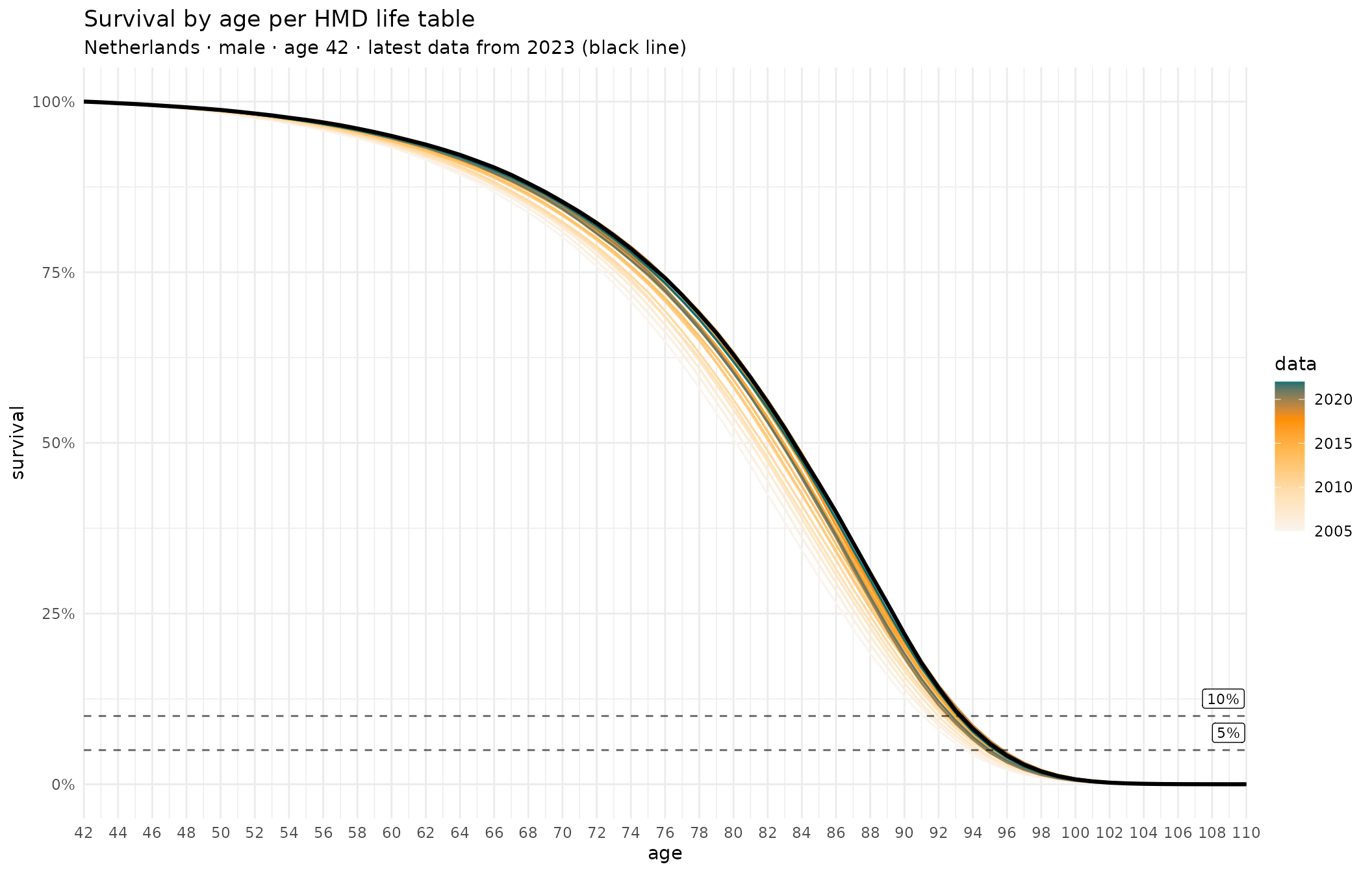

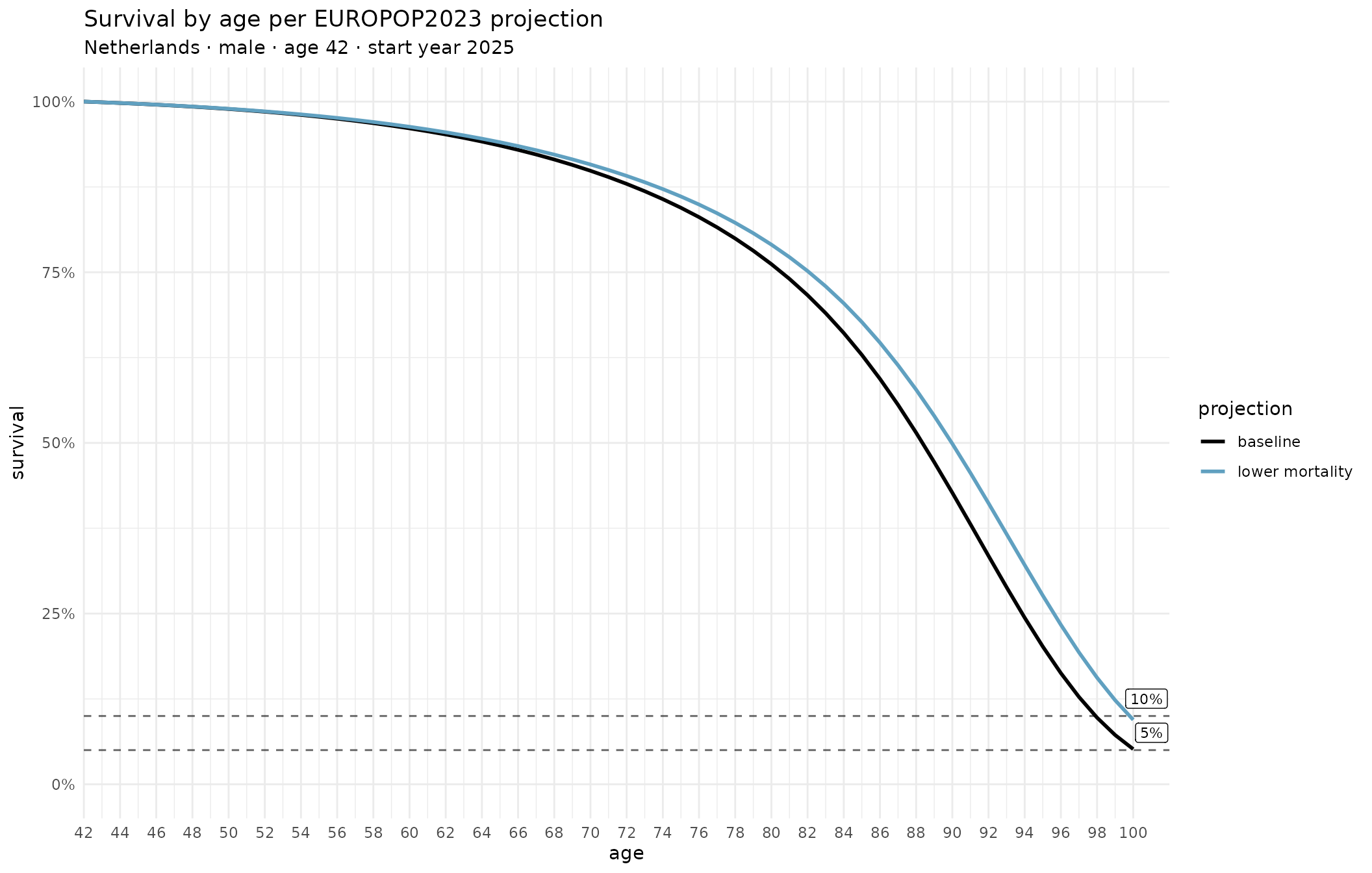
Output

hmd_p

Plot survival chances per EUROPOP23 projections (baseline and lower mortality scenario)

# Dutch male, age 42; use projected age x calendar year mortality starting from 2025

# Table contains both sexes
es <- read_es_aasmr(data_dir)
#> Warning: There were 2 warnings in `mutate()`.
#> The first warning was:
#> ℹ In argument: `Age = dplyr::case_when(...)`.
#> Caused by warning:
#> ! NAs introduced by coercion
#> ℹ Run `dplyr::last_dplyr_warnings()` to see the 1 remaining warning.

# Use Eurostat 'geo' code (2-letter country code)
es_ca <- chance_alive_es_aasmr(es, "NL", "m", 42, 2025) 

# Get a ggplot2 object; 2nd and third argument passed just to label the plot
es_p <- plot_chance_alive_es_aasmr(es_ca, "m", "Netherlands")

# Save SVG file, queue PNG output (or write PNG directly, depending on config)
save_plot("es_plot", es_p, width = 11, height = 7, px_width = 1700)

Output

es_p

Optional: export PNGs via Inkscape

export_pngs()